Density, distribution function, quantile function and random generation for
the beta-binomial distribution with parameters size, prob,
theta, shape1, shape2. This distribution corresponds to
an overdispersed binomial distribution.
Usage
dbetabinom(x, size, prob, theta, shape1, shape2, log = FALSE)

pbetabinom(
  q,
  size,
  prob,
  theta,
  shape1,
  shape2,
  lower.tail = TRUE,
  log.p = FALSE
)

qbetabinom(
  p,
  size,
  prob,
  theta,
  shape1,
  shape2,
  lower.tail = TRUE,
  log.p = FALSE
)

rbetabinom(n, size, prob, theta, shape1, shape2)
Arguments
- x, q
Vector of quantiles.
- size
Number of trials.
- prob
Probability of success on each trial.
- theta
Aggregation parameter (theta = 1 / (shape1 + shape2)).
- shape1, shape2
Shape parameters.
- log, log.p
Logical; if TRUE, probabilities p are given as log(p).
- lower.tail
Logical; if TRUE (default), probabilities are \(P[X \le x]\) otherwise, \(P[X > x]\).
- p
Vector of probabilities.
- n
Number of observations.
Value
dbetabinom gives the density, pbetabinom gives the distribution
function, qbetabinom gives the quantile function and rbetabinom
generates random deviates.
Details
Be aware that in this implementation theta = 1 / (shape1 +
shape2). prob and theta, or shape1 and
shape2 must be specified. if theta = 0, use *binom family
instead.
See also
dbetabinom in the package emdbook
where the definition of theta is different.
Examples
# Compute P(25 < X < 50) for X following the Beta-Binomial distribution
# with parameters size = 100, prob = 0.5 and theta = 0.35:
sum(dbetabinom(25:50, size = 100, prob = 0.5, theta = 0.35))
#> [1] 0.3054911
# When theta tends to 0, dbetabinom outputs tends to dbinom outputs:
sum(dbetabinom(25:50, size = 100, prob = 0.5, theta = 1e-7))
#> [1] 0.5397943
sum(dbetabinom(25:50, size = 100, shape1 = 1e7, shape2 = 1e7))
#> [1] 0.5397944
sum(dbinom(25:50, size = 100, prob = 0.5))
#> [1] 0.5397945
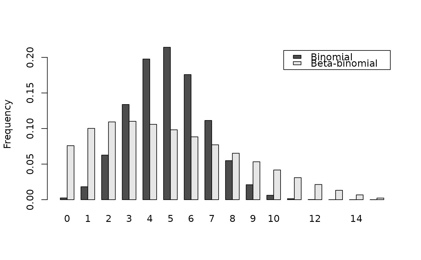
# Example of binomial and beta-binomial frequency distributions:
n <- 15
q <- 0:n
p1 <- dbinom(q, size = n, prob = 0.33)
p2 <- dbetabinom(q, size = n, prob = 0.33, theta = 0.22)
res <- rbind(p1, p2)
dimnames(res) <- list(c("Binomial", "Beta-binomial"), q)
barplot(res, beside = TRUE, legend.text = TRUE, ylab = "Frequency")
 # Effect of the aggregation parameter theta on probability density:
thetas <- seq(0.001, 2.5, by = 0.001)
density1 <- rep(sum(dbinom(25:50, size = 100, prob = 0.5)), length(thetas))
density2 <- sapply(thetas, function(theta) {
sum(dbetabinom(25:50, size = 100, prob = 0.5, theta = theta))
})
plot(thetas, density2, type = "l",
xlab = expression("Aggregation parameter ("*theta*")"),
ylab = "Probability density between 25 and 50 (size = 100)")
lines(thetas, density1, lty = 2)
# Effect of the aggregation parameter theta on probability density:
thetas <- seq(0.001, 2.5, by = 0.001)
density1 <- rep(sum(dbinom(25:50, size = 100, prob = 0.5)), length(thetas))
density2 <- sapply(thetas, function(theta) {
sum(dbetabinom(25:50, size = 100, prob = 0.5, theta = theta))
})
plot(thetas, density2, type = "l",
xlab = expression("Aggregation parameter ("*theta*")"),
ylab = "Probability density between 25 and 50 (size = 100)")
lines(thetas, density1, lty = 2)
