Map Comparison procedure.

mapcomp performs a spatial pattern analysis based on the calculation of a formal distance (the Hellinger distance) between the density map of count or incidence data, and the density map of sampling effort. Statistical tests of spatial homogeneity are based on permutations across sampling sites and on valuable properties of the Hellinger distance.

Usage

mapcomp(data, ...)

# S3 method for data.frame
mapcomp(
  data,
  delta,
  bandwidth,
  nperm = 100,
  edge_correction = FALSE,
  threads = 1,
  verbose = TRUE,
  ...
)

# S3 method for matrix
mapcomp(
  data,
  delta,
  bandwidth,
  nperm = 100,
  edge_correction = FALSE,
  threads = 1,
  verbose = TRUE,
  ...
)

# S3 method for count
mapcomp(
  data,
  delta,
  bandwidth,
  nperm = 100,
  edge_correction = FALSE,
  threads = 1,
  verbose = TRUE,
  ...
)

# S3 method for incidence
mapcomp(
  data,
  delta,
  bandwidth,
  nperm = 100,
  edge_correction = FALSE,
  threads = 1,
  verbose = TRUE,
  ...
)

Arguments

data

A data frame or a matrix with only three columns: the two first ones must be the x and y coordinates of the sampling units, and the last one, the corresponding disease intensity observations. It can also be a count or an incidence object.

...

Additional arguments to be passed to other methods.

delta

Mesh size of the grid over the geographical domain of the sampling units used to compute the integral Hellinger distance between the probability density function of observations and the probability density function of sampling effort.

bandwidth

Bandwidth parameter for smoothing. It allows to test the spatial extent of heterogeneity if any.

nperm

Number of random permutations to assess probabilities.

edge_correction

Apply edge correction to account for the fact that bordering points intrinsically suffer from a lack of neighboring observation sites. FALSE by default.

threads

Number of threads to perform the computations.

verbose

Explain what is being done (TRUE by default).

Value

An object of class mapcomp, which is a list containing the following components:

data	The input data.
coord	The coordinates and normalized intensity for each point of the full grid.
object	The class of data.
bandwidth	The bandwidth parameter.
stat, pval	The statistic and corresponding p-value (see references for more details).

References

Lavigne C, Ricci B, Franck P, Senoussi R. 2010. Spatial analyses of ecological count data: A density map comparison approach. Basic and Applied Ecology. 11:734–742.

Examples

set.seed(123)
my_res <- mapcomp(codling_moths, delta = 1, bandwidth = 11,
                  edge_correction = FALSE, nperm = 20)
my_res
#> Map Comparison analysis (mapcomp)
#> 
#> Call:
#> mapcomp.data.frame(data = codling_moths, delta = 1, bandwidth = 11, 
#>     nperm = 20, edge_correction = FALSE)
#> 
#> Stat: 0.3423 (P = 0.047619)
#> 
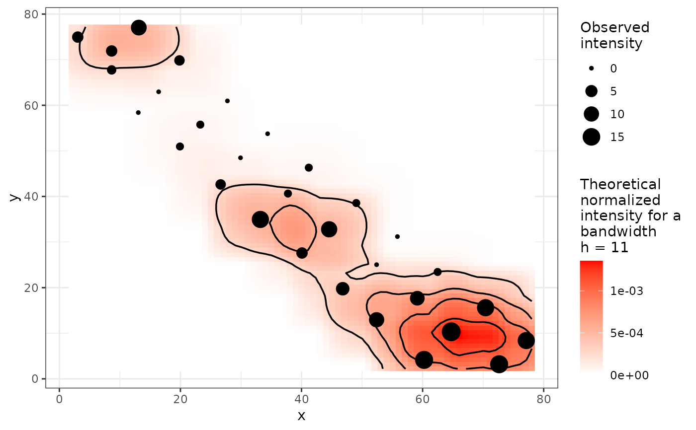
plot(my_res)


set.seed(123)
my_count <- count(codling_moths, mapping(x = xm, y = ym))
my_res <- mapcomp(my_count, delta = 1, bandwidth = 11,
                  edge_correction = FALSE, nperm = 20)
my_res
#> Map Comparison analysis (mapcomp)
#> 
#> Call:
#> mapcomp.count(data = my_count, delta = 1, bandwidth = 11, nperm = 20, 
#>     edge_correction = FALSE)
#> 
#> Stat: 0.3423 (P = 0.047619)
#> 
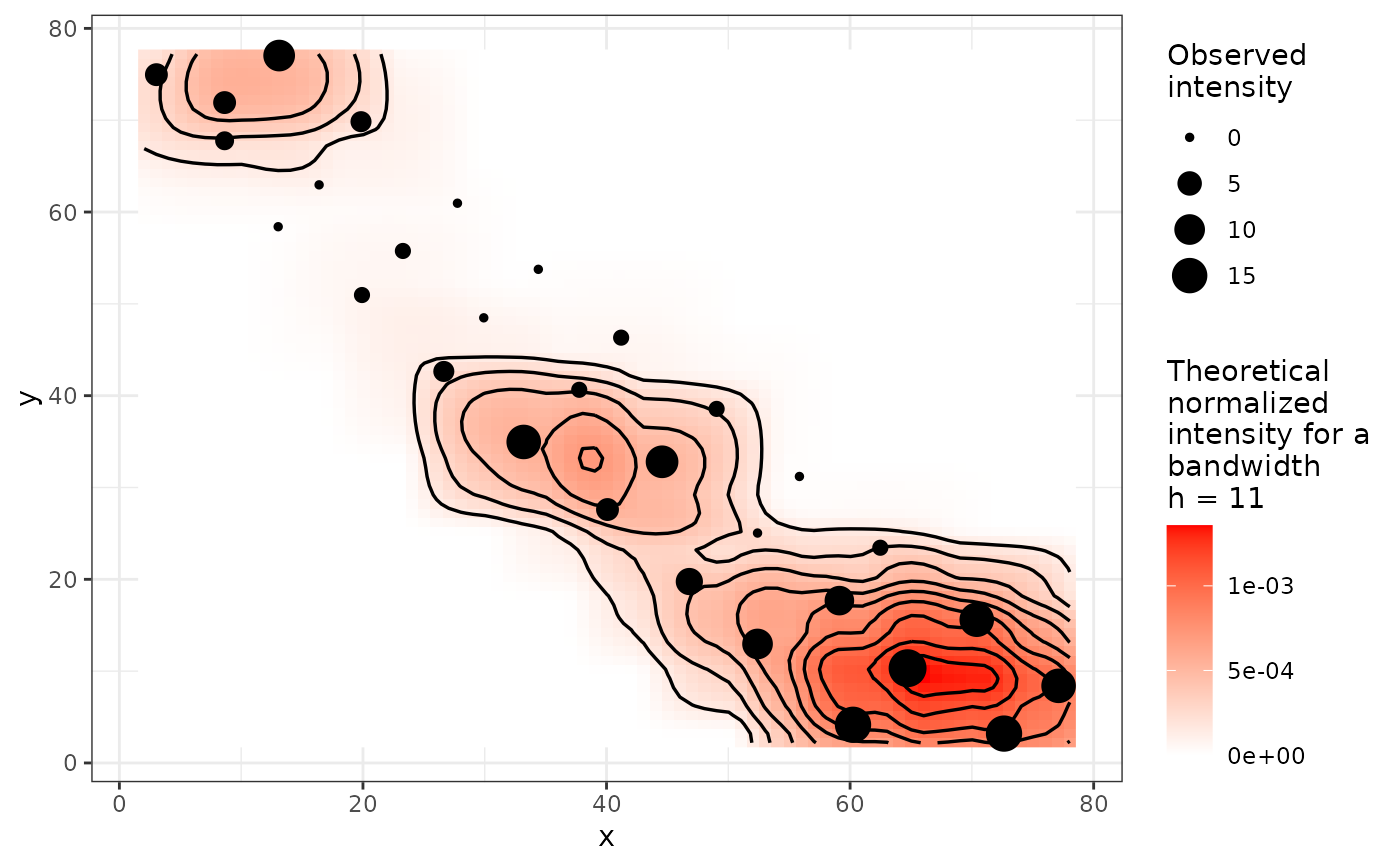
plot(my_res, bins = 10)