sadie performs the SADIE procedure. It computes different indices and
probabilities based on the distance to regularity for the observed spatial
pattern and a specified number of random permutations of this pattern. Both
kind of clustering indices described by Perry et al. (1999) and Li et al.
(2012) can be computed.
Usage
sadie(data, ...)

# S3 method for data.frame
sadie(
  data,
  index = c("Perry", "Li-Madden-Xu", "all"),
  nperm = 100,
  seed = NULL,
  threads = 1,
  ...,
  method = "shortsimplex",
  verbose = TRUE
)

# S3 method for matrix
sadie(
  data,
  index = c("Perry", "Li-Madden-Xu", "all"),
  nperm = 100,
  seed = NULL,
  threads = 1,
  ...,
  method = "shortsimplex",
  verbose = TRUE
)

# S3 method for count
sadie(
  data,
  index = c("Perry", "Li-Madden-Xu", "all"),
  nperm = 100,
  seed = NULL,
  threads = 1,
  ...,
  method = "shortsimplex",
  verbose = TRUE
)

# S3 method for incidence
sadie(
  data,
  index = c("Perry", "Li-Madden-Xu", "all"),
  nperm = 100,
  seed = NULL,
  threads = 1,
  ...,
  method = "shortsimplex",
  verbose = TRUE
)
Arguments
- data
A data frame or a matrix with only three columns: the two first ones must be the x and y coordinates of the sampling units, and the last one, the corresponding disease intensity observations. It can also be a
countor anincidenceobject.- ...
Additional arguments to be passed to other methods.
- index
The index to be calculated: "Perry", "Li-Madden-Xu" or "all". By default, only Perry's index is computed for each sampling unit.
- nperm
Number of random permutations to assess probabilities.
- seed
Fixed seed to be used for randomizations (only useful for checking purposes). Not fixed by default (= NULL).
- threads
Number of threads to perform the computations.
- method
Method for the transportation algorithm.
- verbose
Explain what is being done (TRUE by default).
Details
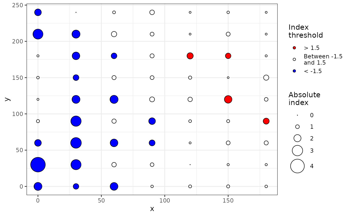
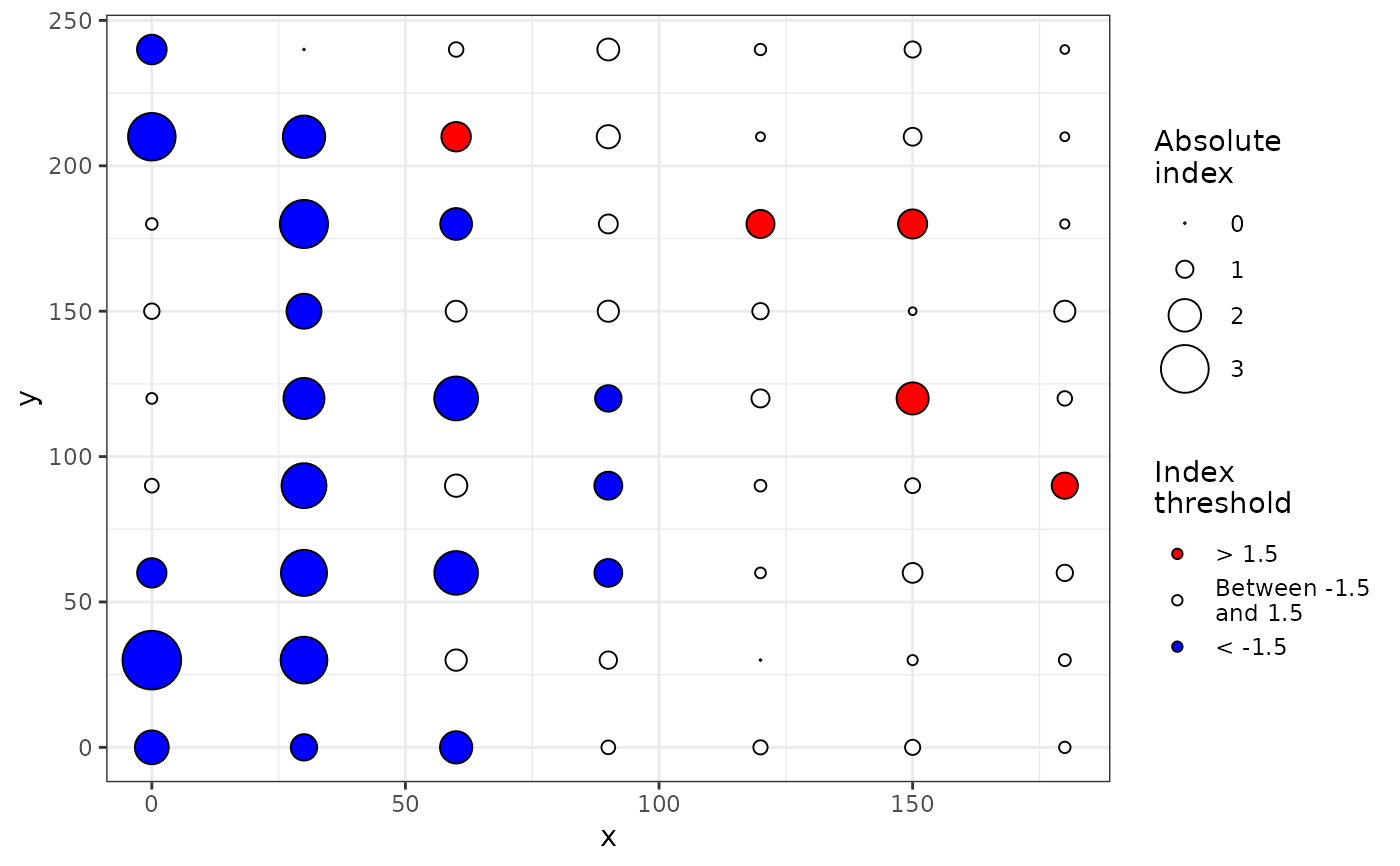
By convention in the SADIE procedure, clustering indices for a donor unit (outflow) and a receiver unit (inflow) are positive and negative in sign, respectively.
References
Perry JN. 1995. Spatial analysis by distance indices. Journal of Animal Ecology 64, 303–314. doi:10.2307/5892
Perry JN, Winder L, Holland JM, Alston RD. 1999. Red–blue plots for detecting clusters in count data. Ecology Letters 2, 106–113. doi:10.1046/j.1461-0248.1999.22057.x
Li B, Madden LV, Xu X. 2012. Spatial analysis by distance indices: an alternative local clustering index for studying spatial patterns. Methods in Ecology and Evolution 3, 368–377. doi:10.1111/j.2041-210X.2011.00165.x
Examples
set.seed(123)
# Create an intensity object:
my_count <- count(aphids, mapping(x = xm, y = ym))
# Only compute Perry's indices:
my_res <- sadie(my_count)
#> Computation of Perry's indices:
my_res
#> Spatial Analysis by Distance IndicEs (sadie)
#>
#> Call:
#> sadie.count(data = my_count)
#>
#> Ia: 1.2569 (Pa = 0.06)
#>
summary(my_res)
#>
#> Call:
#> sadie.count(data = my_count)
#>
#> First 6 rows of clustering indices:
#> x y i cost_flows idx_P idx_LMX prob
#> 1 0 0 0 -148.09142 -2.2522651 NA NA
#> 2 30 0 0 -91.27589 -1.5275799 NA NA
#> 3 60 0 3 -108.16654 -2.1907077 NA NA
#> 4 90 0 7 -40.99681 -0.6336085 NA NA
#> 5 120 0 9 30.00000 0.7628231 NA NA
#> 6 150 0 1 -42.31033 -0.7946351 NA NA
#>
#> Summary indices:
#> overall inflow outflow
#> Perry's index 1.309858 -1.458153 1.119927
#> Li-Madden-Xu's index NA NA NA
#>
#> Main outputs:
#> Ia: 1.2569 (Pa = 0.06)
#>
#> 'Total cost': 1061.153
#> Number of permutations: 100
#>
plot(my_res)
 plot(my_res, isoclines = TRUE)
 set.seed(123)
# Compute both Perry's and Li-Madden-Xu's indices (using multithreading):
my_res <- sadie(my_count, index = "all", threads = 2, nperm = 20)
#> Computation of Perry's indices:
#> Computation of Li-Madden-Xu's indices:
my_res
#> Spatial Analysis by Distance IndicEs (sadie)
#>
#> Call:
#> sadie.count(data = my_count, index = "all", nperm = 20, threads = 2)
#>
#> Ia: 1.3517 (Pa = 0.05)
#>
summary(my_res)
#>
#> Call:
#> sadie.count(data = my_count, index = "all", nperm = 20, threads = 2)
#>
#> First 6 rows of clustering indices:
#> x y i cost_flows idx_P idx_LMX prob
#> 1 0 0 0 -148.09142 -2.0856425 -3.0083225 0.04761905
#> 2 30 0 0 -91.27589 -1.5994304 -1.5545829 0.23809524
#> 3 60 0 3 -108.16654 -1.9837172 -1.9703605 0.14285714
#> 4 90 0 7 -40.99681 -0.7734811 -0.7590137 0.66666667
#> 5 120 0 9 30.00000 0.8051948 0.8750000 0.09523810
#> 6 150 0 1 -42.31033 -0.8651327 -0.8268594 0.57142857
#>
#> Summary indices:
#> overall inflow outflow
#> Perry's index 1.385343 -1.558203 1.149058
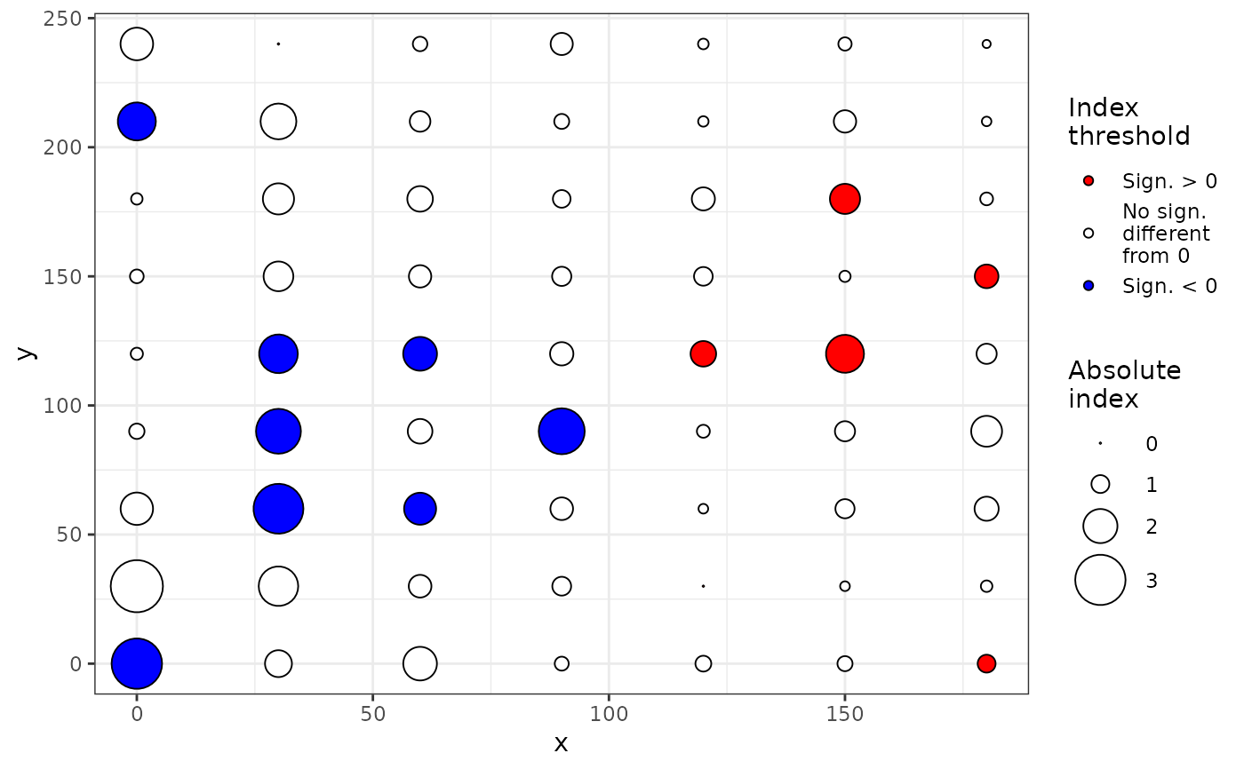
#> Li-Madden-Xu's index 1.317835 -1.431426 1.205459
#>
#> Main outputs:
#> Ia: 1.3517 (Pa = 0.05)
#>
#> 'Total cost': 1061.153
#> Number of permutations: 20
#>
plot(my_res) # Identical to: plot(my_res, index = "Perry")
set.seed(123)
# Compute both Perry's and Li-Madden-Xu's indices (using multithreading):
my_res <- sadie(my_count, index = "all", threads = 2, nperm = 20)
#> Computation of Perry's indices:
#> Computation of Li-Madden-Xu's indices:
my_res
#> Spatial Analysis by Distance IndicEs (sadie)
#>
#> Call:
#> sadie.count(data = my_count, index = "all", nperm = 20, threads = 2)
#>
#> Ia: 1.3517 (Pa = 0.05)
#>
summary(my_res)
#>
#> Call:
#> sadie.count(data = my_count, index = "all", nperm = 20, threads = 2)
#>
#> First 6 rows of clustering indices:
#> x y i cost_flows idx_P idx_LMX prob
#> 1 0 0 0 -148.09142 -2.0856425 -3.0083225 0.04761905
#> 2 30 0 0 -91.27589 -1.5994304 -1.5545829 0.23809524
#> 3 60 0 3 -108.16654 -1.9837172 -1.9703605 0.14285714
#> 4 90 0 7 -40.99681 -0.7734811 -0.7590137 0.66666667
#> 5 120 0 9 30.00000 0.8051948 0.8750000 0.09523810
#> 6 150 0 1 -42.31033 -0.8651327 -0.8268594 0.57142857
#>
#> Summary indices:
#> overall inflow outflow
#> Perry's index 1.385343 -1.558203 1.149058
#> Li-Madden-Xu's index 1.317835 -1.431426 1.205459
#>
#> Main outputs:
#> Ia: 1.3517 (Pa = 0.05)
#>
#> 'Total cost': 1061.153
#> Number of permutations: 20
#>
plot(my_res) # Identical to: plot(my_res, index = "Perry")
 plot(my_res, index = "Li-Madden-Xu")
 set.seed(123)
# Using usual data frames instead of intensity objects:
my_df <- aphids[, c("xm", "ym", "i")]
sadie(my_df)
#> Computation of Perry's indices:
#> Spatial Analysis by Distance IndicEs (sadie)
#>
#> Call:
#> sadie.data.frame(data = my_df)
#>
#> Ia: 1.2569 (Pa = 0.06)
#>
set.seed(123)
# Using usual data frames instead of intensity objects:
my_df <- aphids[, c("xm", "ym", "i")]
sadie(my_df)
#> Computation of Perry's indices:
#> Spatial Analysis by Distance IndicEs (sadie)
#>
#> Call:
#> sadie.data.frame(data = my_df)
#>
#> Ia: 1.2569 (Pa = 0.06)
#>